How to make a pivot table, step by step
Turn a long list of sales into a clear summary by region and quarter. A beginner friendly pivot table walkthrough with grouping, totals and percentages.
A pivot table answers questions like "how much did each region sell per quarter?" without a single formula. You give it a list of records, tell it which column goes down the side, which goes across the top and which numbers to add up, and it builds the summary for you.
This guide walks through a complete example in SheetsBat, from a raw order list to a revenue by region and quarter table with percentages and a chart. The steps use the free Sales dashboard template, so you can follow along with the same numbers.
What a pivot table needs
Pivot tables work on data shaped like a list:
- One header row with a name in every column (Date, Region, Rep, Revenue and so on).
- One row per record, such as one row per order.
- No blank rows or subtotal rows inside the data.
- Consistent values in each column: real dates in the date column, numbers in the number columns.
The Data sheet of the Sales dashboard template already looks like this. It holds 103 sample orders for an outdoor gear shop, in a table named Sales with the columns Date, Order, Region, Rep, Product, Units, Price and Revenue.
Step 1: open the Create pivot table panel
- Open the workbook and go to the sheet with your data.
- Click any cell inside the data.
- Choose Insert, then Pivot table. The same command is also in the Data menu.
The Create pivot table panel opens on the right. SheetsBat fills in the Data range from the cell you clicked. When the data is a table, it says so: "Uses table Sales, so new rows are included automatically."
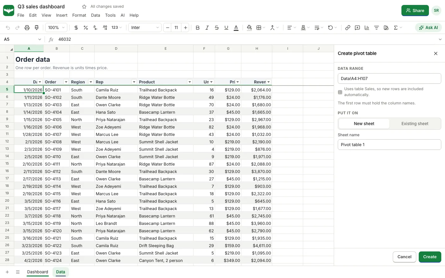
- Under Put it on, choose New sheet (the default) or Existing sheet if you want the summary next to other work. A new sheet gets a name such as "Pivot table 1", which you can change in the Sheet name box.
- Click Create.
You now have an empty pivot table and the field list. Nothing is calculated until you add fields.
Step 2: add fields to rows, columns and values
The panel lists every column of your data under Fields, with a search box for wide tables. Below are four zones: Rows, Columns, Values and Filters. You can drag a field into a zone, or click a field and choose Add to rows, Add to columns, Add to values or Add to filters.
For revenue by region and quarter:
- Add Region to Rows. Each region becomes a row.
- Add Date to Columns. SheetsBat recognises the dates and groups them, starting with one column per month.
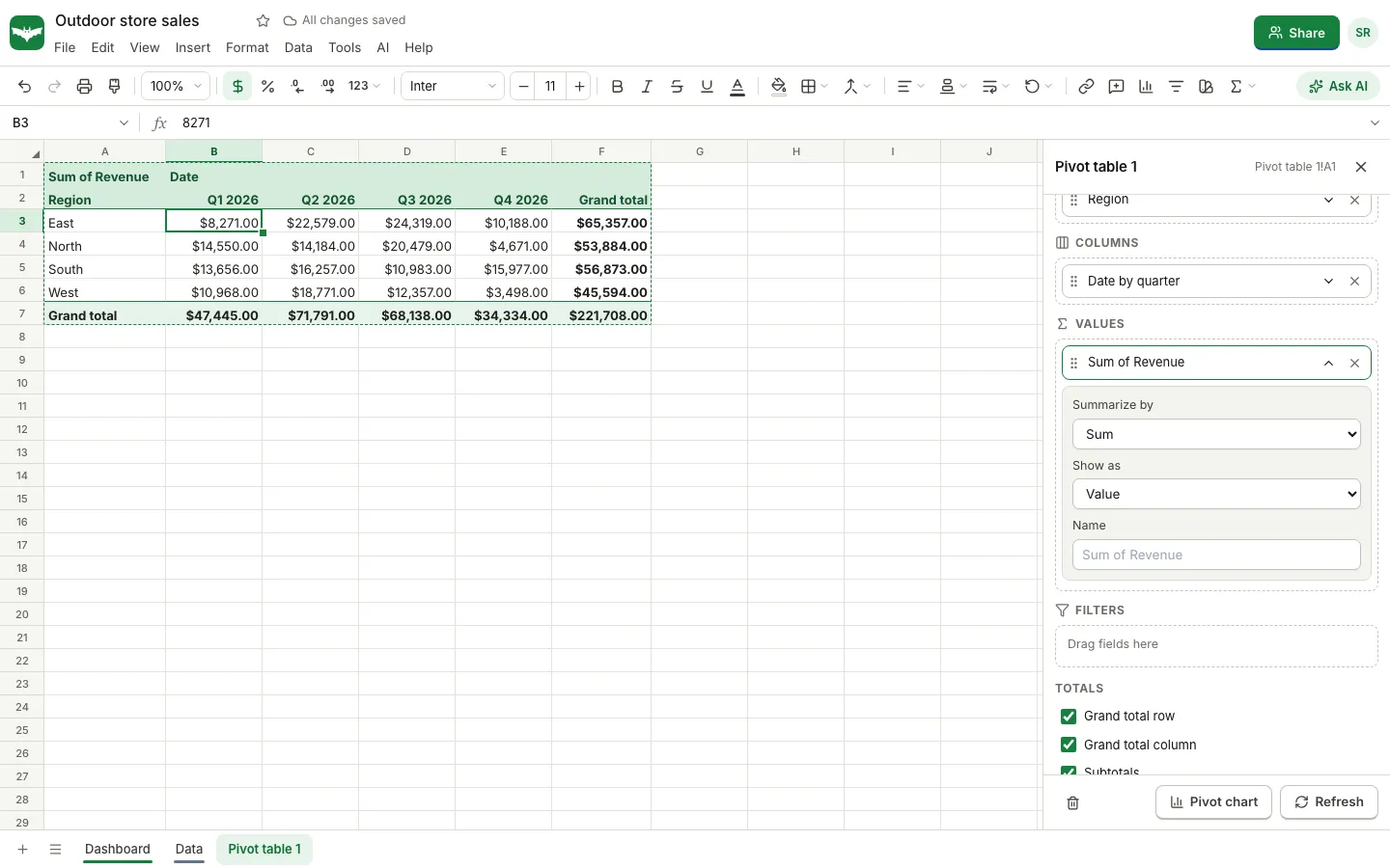
- Add Revenue to Values. Number fields are summed by default, so the chip reads "Sum of Revenue".
The table appears on the sheet straight away, with a grand total row and a grand total column.
Step 3: group dates by quarter
Twelve month columns are a lot to read. To group by quarter:
- In the Columns zone, click the Date by month chip to open its options.
- Set Group dates by to Quarter.
The other choices are Year, Month, Year and month, Day of week and Day, or No grouping. The chip now reads "Date by quarter", and the table shrinks to one column per quarter.
Each row and column chip also has a Sort setting. You can sort labels A to Z or Z to A, or sort by a value, for example to put the region with the highest revenue at the top.
Step 4: change how values are summarised
Click the Sum of Revenue chip in Values to see its options:
- Summarize by: Sum, Count, Count numbers, Count unique, Average, Min, Max, Product, Standard deviation or Variance.
- Show as: Value, % of grand total, % of row total, % of column total or Running total.
- Name: the label shown in the table, for example "Revenue" instead of "Sum of Revenue".
A few useful combinations:
| Question | Field in Values | Summarize by | Show as |
|---|---|---|---|
| How much did each region sell? | Revenue | Sum | Value |
| What share of the year was each region? | Revenue | Sum | % of grand total |
| How many orders did each rep close? | Order | Count | Value |
| How many different products did each region buy? | Product | Count unique | Value |
| What was the typical order size? | Revenue | Average | Value |
| How did revenue build up over the year? | Revenue | Sum | Running total |
You can add the same field to Values more than once. Add Revenue twice, show the first as a value and the second as % of row total, and you see both the dollars and each quarter's share of the region's year.
Step 5: filter the pivot table
Drag a field into Filters to limit what the pivot counts. For example, add Product to Filters and untick everything except one product to see where it sells best. The filter has its own search box and a Select all option.
Step 6: totals, subtotals and layout
Under Totals at the bottom of the panel you can switch the Grand total row, the Grand total column and Subtotals on or off. Subtotals matter when you put two fields in Rows, such as Region and then Rep: each region gets its own subtotal line under its reps.
To change the order of fields in a zone, open a chip and use Move up or Move down, or drag the chips.
Step 7: add a pivot chart
Click Pivot chart at the bottom of the panel. SheetsBat adds a chart next to the pivot table that follows its layout, such as a column chart of revenue per region with one series per quarter. You can change the chart type and style like any other chart.
Keeping the pivot table up to date
The output of a pivot table is written into the sheet as ordinary cells, so it saves, prints, exports to Excel and syncs to collaborators like anything else. SheetsBat keeps pivot tables fresh when their source data changes, and there is a Refresh button in the panel if you want to recalculate on demand.
To edit an existing pivot table later, click any cell inside it and choose Edit pivot table. The same panel opens with your fields in place. Change next to the data source lets you point the pivot at a different range.
Pivot tables without the panel
If you prefer formulas, SheetsBat also supports the GROUPBY and PIVOTBY functions, which return a summary as a spilling array. For example:
=PIVOTBY(Sales[Region], Sales[Product], Sales[Revenue], SUM)returns revenue with regions down the side and products across the top. Formula summaries are handy inside dashboards, while the pivot panel is quicker for exploring.
Common problems
- Dates show as numbers or do not group. Some cells in the date column are text. Convert them to real dates and refresh.
- Revenue is counted instead of summed. The column contains text values, such as a dollar amount typed with a note. Clean the column, then set Summarize by back to Sum.
- New rows are missing. The pivot uses a fixed range rather than a table. Turn the data into a table, or use Change to widen the range.
- The pivot needs more room. If the summary would overwrite nearby cells, SheetsBat asks before replacing them, so put the pivot on its own sheet when in doubt.
Share the result
When the summary is ready, use the Share button to invite your team or create a view only link. Everyone sees the same numbers, and people with edit access can explore the pivot with you live. Our guide to how to co-edit a spreadsheet in real time shows how that works, and if you need to pull single values from the same data, see XLOOKUP vs VLOOKUP with examples. Bookkeepers who build pivots from exported ledgers may also like our guide to giving your accountant access to your books.
Frequently asked questions
What is a pivot table used for?
A pivot table summarises a list of records by the categories you choose, such as total sales by region and month, orders per rep or average order value per product, without writing formulas.
Why is my pivot table counting instead of summing?
A pivot field counts when some of its cells hold text. Make sure every cell in the number column is a real number, then open the value chip and set Summarize by to Sum.
Does a pivot table update when I add new data?
In SheetsBat, yes when the pivot is built on a table: new rows in the table are included. If you used a plain range, widen it with Change or turn the data into a table first.
Can I group dates by month or quarter?
Yes. Open the date field's chip in Rows or Columns and set Group dates by to Year, Quarter, Month, Year and month, Day of week or Day.
Is the SheetsBat pivot table free?
Yes. Pivot tables, pivot charts, grouping and percentages are part of the Free plan. SheetsBat Free includes 25 workbooks with up to 500,000 cells each.